Pieter van Gelder TU Delft

Presentatie over: "Pieter van Gelder TU Delft"— Transcript van de presentatie:

1 Pieter van Gelder TU Delft
Cursus Betonvereniging 25 Oktober Design-by-Testing Beslistheorie Tijdsafhankelijk falen Pieter van Gelder TU Delft

2 Sterkte - design by testing
NEN 6700, par. 7.2 Experimentele modellen Rekening houden met: Vereenvoudigingen experimenteel model Onzekerheden m.b.t. lange-duur effecten Representatieve steekproeven Statistische onzekerheden Wijze van bezwijken (bros/taai) Eisen m.b.t. detaillering Bezwijkmechanismen Belastingen besproken. Nu sterkte. Redelijk dichtgetimmerd in de norm. Uitzondering: nieuwe materialen/componenten. Daarin kan je al snel met experimenteel werk te maken krijgen.

3 Voorbeeld Nieuw anker voor bevestiging gevelelementen.
Onder horizontale (wind-)belasting Mogelijke bezwijkmechanismen: spreidanker in beton bezwijkt anker zelf bezwijkt ankerdoorn breekt uit

4 Voorbeeld Sterkte anker meten in proefopstelling. Resultaten (in N):
4897 2922 3700 4856 3221 Wat is de karakteristieke waarde (5%)? Betrek ze in de disussie.

5 Statistische zekerheid
Situatie: Sterkte R normaal verdeeld Veel metingen Formule voor sterkte: u : standaard normaal verdeelde variabele mR: steekproefgemiddelde SR: standaarddeviatie uit steekproef R = m + u S R R

6 Tabel normale verdeling

7 Statistische onzekerheid
Situatie: Sterkte R normaal verdeeld Weinig metingen (n) Gemiddelde onbekend Standaarddeviatie onbekend Bayesiaanse statistiek: n : aantal metingen tn-1 : standaard student verdeelde variabele met n-1 vrijheidsgraden mR: steekproefgemiddelde SR: standaarddeviatie uit steekproef 1 R = m + t S 1 + R n - 1 R n

8 Student t verdeling

9 Statistische onzekerheid
Situatie: Sterkte R normaal verdeeld Weinig metingen (n) Gemiddelde onbekend Standaarddeviatie bekend Bayesiaanse statistiek: n : aantal metingen u : standaard normaal verdeelde variabele mR: steekproefgemiddelde sR: bekende standaarddeviatie 1 R = m + u s 1 + R R n

10 Voorbeeld Gegeven: 3 metingen: 88, 95 en 117 kN
Bekende standaarddeviatie 15 kN Vraag: Bereken de karakteristieke waarde (5%)

11 Voorbeeld Gegeven: 3 metingen: 88, 95 en 117 kN
Onbekende standaarddeviatie Vraag: Bereken de karakteristieke waarde (5%)

12 Voorbeeld Gegeven: 100 metingen steekproefgemiddelde 100 kN
Onbekende standaarddeviatie, uit steekproef: 15 kN Vraag: Bereken de karakteristieke waarde (5%)

13 Voorbeeld

14 Voorbeeld

15 Beslistheorie

16 Rationeel beslissen: ijscoman
P{zon} = P{regen} = 0.5 regen € 0 ijs zon € 1000 regen € 2000 patat zon € -500

17 Rationeel beslissen: ijscoman
P{zon} = P{regen} = 0.5 Verwachte opbrengst: regen € 0 ijs 0 * * 0.5 = 500 zon € 1000 regen € 2000 patat 2000 * * 0.5 = 750 zon € -500

18 Irrationeel beslissen
Risico-avers voorbeeld uitwerken op bord

19 Definitie van risico Risico = kans x gevolg

20 Matrix of risks Small prob, small event Small prob, large event
Large prob, small event Large prob, large event

21

22 Evaluating the risk Testing the risk to predetermined standards
Testing if the risk is in balance with the investment costs

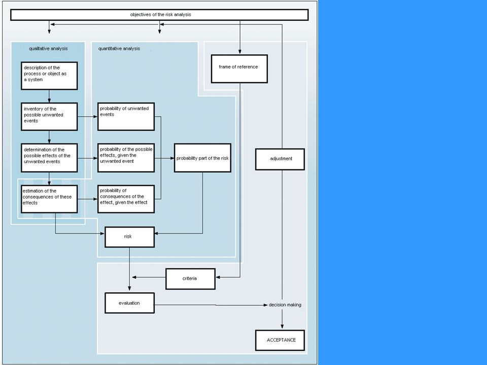
23 Decision-making based on risk analysis
Recording different variants, with associated risks, costs and benefits, in a matrix or decision tree, serves as an aid for making decisions. With this, the optimal selection can be made from a number of alternatives.

24 Deciding under uncertainties
Modern decision theory is based on the classic “Homo Economicus” model has complete information about the decision situation; knows all the alternatives; knows the existing situation; knows which advantages and disadvantages each alternative provides, be it in the form of random variables; strives to maximise that advantage.

25 But in reality The decision maker: does not know all the alternatives;
does not know all the effects of the alternatives; does not know which effect each alternative has.

26 A decision model A: the set of all possible actions (a), of which one must be chosen; N: the set of all (natural) circumstances (θ); Ω: the set of all possible results (ω), which are functions of the actions and circumstances: ω = f(a, θ).

27 Example 4.1 Suppose a person has EUR 1000 at his disposal and is given the choice to invest this money in bonds or in shares of a given company. The decision model consists of: a1 = investing in shares a2 = investing in bonds θ1 = company profit # 5 % θ2 = 5 % <  company profit # 10 % θ3 = company profit > 10 % ω1 = return (0 % ‑ 2 %) = ‑2 % per annum ω2 = return (3 % ‑ 2 %) =  1 % per annum ω3 = return (6 % ‑ 2 %) =  4 % per annum

28 Decision tree (example 4.1)

29 Results space Utility space

30 Likelihood of the circumstances

31 From discrete to continuous decision models

32 Dijkhoogte bepaling Op bord uitwerken

33 Tijdsafhankelijke faalkansen
Door veroudering is onderhoud noodzakelijk: Onderhoudsmodellen

34 Levensduur T: is een stochastische variabele

35 J.K. Vrijling and P.H.A.J.M. van Gelder, The effect of inherent uncertainty in time and space on the reliability of flood protection, ESREL'98: European Safety and Reliability Conference 1998, pp , June 1998, Trondheim, Norway.

36 Haringvliet outlet sluices
Modellering Lifetime distribution for one component Time start t Replacement strategies of large numbers of similar components in hydraulic structures

37 Voorbeeld “leeftijd van mensen”: stochastische variable Lmens
Lmens ~ N(78,6) of EXP(76,8) P(Lmens >90)=...? P(Lmens >90| Lmens >89)= P(Lmens >90)/P(Lmens >89)=... Uitwerken op bord Vervolgens: Modelvorming voor algemene situatie

38 Verwachte resterende levensduur als functie van reeds bereikte leeftijd

39 Hazard rate population in S-Africa: f(t) / [1 - F(t) ]

40 T = time to failure The Hazard Rate, or instantaneous failure rate is defined as: h(t) = f(t) / [1 - F(t) ] = f(t) / R(t) f(t) probability density function of time to failure, F(t) is the Cumulative Distribution Function (CDF) of time to failure, R(t) is the Reliability function (CCDF of time to failure). From:     f(t) = d F(t)/dt , it follows that: h(t) dt = d F(t) / [1 - F(t) ] = - d R(t) / R(t) = - d ln R(t)

41 Integrating this expression between 0 and T yields an expression relating the Reliability function R(t) and the Hazard Rate h(t):

42 Bathtub Curve

43 Constant Hazard Rate The most simple Hazard Rate model is to assume that: h(t) = λ , a constant. This implies that the Hazard or failure rate is not significantly increasing with component age. Such a model is perfectly suitable for modeling component hazard during its useful lifetime. Substituting the assumption of constant failure rate into the expression for the Reliability yields: R(t) = 1 - F(t) = exp (- λt) This results in the simple exponential probability law for the Reliability function.

44 Non-Constant Hazard Rate
One of the more common non-constant Hazard Rate models used for evaluation of component aging phenomenon, is to assume a Weibull distribution for the time to failure: Using the definition of the Hazard function and substituting in appropriate Weibull distribution terms yields: h(t) = f(t) / [1 - F(t) ] = β t β -1 / t β

45 For the specific case of: β = 1
For the specific case of:  β = 1.0 , the Hazard Rate h(t) reverts back to the constant failure rate model described above, with:  t = 1/  λ . The specific value of the β parameter determines whether the hazard is increasing or decreasing.

46 β values, 0.5, 1.0, and 1.5.

47 β values, 0.5, 1.0, and 1.5.

48 Maintenance in Civil Engineering
Many design and build projects in the past Nowadays many maintenance projects

49 Good Detoriation Model? State dependent Contains Effect of Loading?
Consequence of failure Corrective Maint. Use Time Load large no small yes no yes

50 Hydraulic Engineering
corrective maintenance is not advised in view of the risks involved preventive maintenance time based failure based load based resistance based

51 repair resistance Failure load based failure time repair resistance
Ro resistance load Failure based failure time repair Ro resistance load Time based Δt time repair Ro resistance load cum. load Load based time repair Ro load Rmin Resistance based time

52 Dike Settlement S.L.S h0 – A ln t = h(t) U.L.S. h(t) – HW R,S h0 hmin
time topt R,S h0 hmin S

53 Condition based maintenance
Inspection good Repair bad

54 Maintenance A case study Some concepts

55 Maintenance strategies
of large numbers of similar components in hydraulic structures

56 Introduction Maintenance  replacement

57 Introduction Large numbers of similar components
Maintenance  replacement Large numbers of similar components

58 Introduction Large numbers of similar components
Maintenance  replacement Large numbers of similar components

59 Introduction Large numbers of similar components
Maintenance  replacement Large numbers of similar components Same lifetime-distribution Same age Same function

60 Variables of a replacement scenario
Modelling Case study Conclusions Modellering Variables of a replacement scenario Start date of the (start) replacements Replacement interval (t) Number of preventive ( ) replacements Time start t

61 Finding the optimal strategy
Modelling Case study Conclusions Modellering Finding the optimal strategy Balance between risk costs and costs of preventive replacements Replacement capacity Capacity of the supplier

62 Probability of failure for different scenarios
Modelling Case study Conclusions Casestudie Probability of failure for different scenarios

63 The Concept of Availability
Reliability Maintainability Availability

64 Maintainability Maintainability is the probability that a process or a system that has failed will be restored to operation effectiveness within a given time. M(t) = 1 - e-mt where m is repair (restoration) rate

65 Availability Availability is the proportion of the process or system “Up-Time” to the total time (Up + Down) over a long period. Up-Time Up-Time + Down-Time Availability =

66 System Operational States
B1 B2 B3 Up t Down A1 A2 A3 Up: System up and running Down: System under repair

67 Mean Time To Fail (MTTF)
MTTF is defined as the mean time of the occurrence of the first failure after entering service. B1 + B2 + B3 3 MTTF = B1 B2 B3 Up t Down A1 A2 A3

68 Mean Time Between Failure (MTBF)
MTBF is defined as the mean time between successive failures. (A1 + B1) + (A2 + B2) + (A3 + B3) 3 MTBF = B1 B2 B3 Up t Down A1 A2 A3

69 Mean Time To Repair (MTTR)
MTTR is defined as the mean time of restoring a process or system to operation condition. A1 + A2 + A3 3 MTTR = B1 B2 B3 Up t Down A1 A2 A3

70 Availability Availability is defined as: Up-Time Up-Time + Down-Time
Availability is normally expressed in terms of MTBF and MTTR as: MTBF MTBF + MTTR A =

71 Reliability/Maintainability Measures
Reliability R(t) (Failure Rate) l = 1 / MTBF R(t) = e-lt Maintainability M(t) (Maintenance Rate) m = 1 / MTTR M(t) = 1 - e-mt

72 Types of Redundancy Active Redundancy Standby Redundancy

73 Active Redundancy A Input Output B Divider
Both A and B subsystems are operative at all times Note: the dividing device is a Series Element

74 Standby Redundancy A Input Output B Switch Standby
The standby unit is not operative until a failure-sensing device senses a failure in subsystem A and switches operation to subsystem B, either automatically or through manual selection.

75 Series System ps = p1 + p2 +……. + pn - (-1)n joint probabilities
Input A1 A2 An Output ps = p1 + p2 +……. + pn - (-1)n joint probabilities For identical and independent elements: ps ~ 1 - (1-p)n < np (>p) ps : Probability of system failure pi : Probability of component failure

76 Parallel System ps = p1.p2 … pn A Input Output B Multiplicative Rule
ps : Probability of system failure

77 Series / Parallel System
Input Output C B1 B2

78 System with Repairs qs = ( 3l + m )/ ( 2l2 ) l << m
Let MTBF = q and system MTBF = qs A Input Output B For Active Redundancy (Parallel or duplicated system) qs = ( 3l + m )/ ( 2l2 ) l << m qs = m / 2l2 = MTBF2 / 2 MTTR

79 qs = ( 2l + m )/ (l2 ) qs = m / l2 = MTBF2 / MTTR A Input Output B
SW Output B Switch Standby Note: The switch is a series element, neglect for now. Note: The standby system is normally inactive. For Standby Redundancy qs = ( 2l + m )/ (l2 ) qs = m / l2 = MTBF2 / MTTR

80 System without Repairs
For systems without repairs, m = 0 For Active Redundancy qs = ( 3l + m )/ ( 2l2 ) qs = 3l / ( 2l2 ) = 3 / ( 2l ) qs = (3/2) q where q = 1/l qs = 1.5 MTBF For Standby Redundancy qs = ( 2l + m )/ (l2 ) qs = 2l/ l2 = 2/ l qs = 2q where q = 1/l qs = 2 MTBF

81 Summary Type With Repairs Without Repairs Active MTBF2 / 2 MTTR
Standby MTBF2 / MTTR 2 MTBF Redundancy techniques are used to increase the system MTBF