Caput Biodiversiteit 2004 Philippine Vergeer Jan van Groenendael.

Presentatie over: "Caput Biodiversiteit 2004 Philippine Vergeer Jan van Groenendael."— Transcript van de presentatie:

1 Caput Biodiversiteit 2004 Philippine Vergeer Jan van Groenendael

2 Caput biodiversiteit colleges 5+6 De paradox van biodiversiteit

3 biodiversiteitsparadoxen
1 Biodiversiteit is een continue stijgende functie van de tijd (met enkele onderbrekingen) 2 Biodiversiteit is functioneel in hoge mate redundant 3 Biodiversiteit is theoretisch tenminste onwaarschijnlijk

4 Diversiteit door de tijd

5 biodiversiteitsparadoxen
1 Biodiversiteit is een continue stijgende functie van de tijd (met enkele onderbrekingen) 2 Biodiversiteit is functioneel in hoge mate redundant 3 Biodiversiteit is theoretisch tenminste onwaarschijnlijk

6 Soortenrijkdom en biomassa

7 Soortenrijkdom en ecosysteemfunctie
After Tilman

8 Eigenschappen

9 Endemisme vs diversiteit
P<0.0001 % endemics No. species

10 Sleutelsoorten

11 Abundantie vs importantie
dominante Abundantie (gewicht/oppervlakte meeste organisme functionele groepering nuttig zeldzaam & onbelangrijk sleutel- soorten Functionele importantie (effect op productiviteit van systeem)

12 biodiversiteitsparadoxen
1 Biodiversiteit is een continue stijgende functie van de tijd (met enkele onderbrekingen) 2 Biodiversiteit is functioneel in hoge mate redundant 3 Biodiversiteit is theoretisch tenminste onwaarschijnlijk

13 Sinds Darwin worden interacties tussen soorten doorgaans gedacht vanuit een perspectief van competitie, “Survival of the fittest” Dit heeft vergaande gevolgen gehad voor de ecologische theorievorming over biodiversiteit in de 20ste eeuw

14 Een populatie groeit naar een draagkracht toe:
P.F. Verhulst 1838 Notice sur la loi que la population suit dans son acroissement Correspondances Mathematiques et Physiques Logistische groei: Een populatie groeit naar een draagkracht toe: dN/dt = rN (K-N)/K r = intrinsieke groeisnelheid N = populatiegrootte K = draagkracht: ‘carrying capacity’

15 Interspecifieke competitie: interactie tussen 2 soorten
Theoretische biologen, ontwikkelden het logistische model voor populatiegroei en koppelden dit aan het effect van interspecifieke concurrentie ‘het Lotka-Volterra model’ Alfred James Lotka Vito Volterra

16 Het Lotka-Volterra model
Logistische groei: dN/dt = rN (K-N)/K Nu 2 soorten: soort 1 (met r1, N1 en K1) soort 2 (met r2, N2 en K2) Er is competitie tussen de 2 soorten: een competitie-coefficient:  12 de last die soort 1 van soort 2 ondervindt 21 de last die soort 2 van soort 1 ondervindt

17 Het Lotka-Volterra model
Dat geeft voor soort 1: dN1/dt = r1N1 (K1-N1- 12 N2)/ K1 Dat geeft voor soort 2: dN2/dt = r2N2 (K2-N2- 21 N1)/ K2 Onder welke omstandigheden neemt soort 1 toe/af en onder welke omstandigheden soort 2? Als dN1/dt = 0 blijft soort 1 gelijk Als dN2/dt = 0 blijft soort 2 gelijk (het berekenen van de ‘nul-isoclines’)

18 Het Lotka-Volterra model
Dat geeft voor soort 1: dN1/dt = r1N1 (K1-N1- 12 N2)/ K1 dN1/dt = 0  r1N1 (K1-N1- 12 N2)/ K1 = 0 N1 = K1- 12 N2 = 0 N1 = K1 en N2 = K1 /12

19 Het Lotka-Volterra model
Dat geeft voor soort 2: dN2/dt = r2N2 (K2-N2- 21 N1)/ K2 dN2/dt = 0  r2N2 (K2-N2- 21 N1)/ K2 = 0 N2 = K2- 21 N1 = 0 N2 = K2 en N1 = K2 /21

20 Het Lotka-Volterra model

21 Het Lotka-Volterra model:
1 stabiel evenwichten 3 instabiele evenwichten

22 In 1934 testte de russische ecoloog Georgii Frantsevich Gause (geb
In 1934 testte de russische ecoloog Georgii Frantsevich Gause (geb.1910) deze theorieën met laboratorium proeven met 2 aan elkaar verwante pantoffeldiertjes (Paramecium aurelia en Paramecium caudatum) De theorieën bleken te kloppen:

23 Georgii Frantsevich Gause (geb.1910)
2 soorten met gelijke behoeftes (zoals bijv. voedsel) kunnen niet in dezelfde ruimte samenleven: de een zal de ander ‘weg-concurreren’: ‘competitive exclusion principle’ ‘limiting similarity principle’ Ook wel ‘Gause’s exclusion principle’ Georgii Frantsevich Gause (geb.1910)

24 Lotka-Volterra en het ‘competitive exclusion principle’ zijn sterk gerelateerd aan het ‘ecologisch niche concept’ ecologische niche: het totaal van alles wat een organisme gebruikt van de biotische en abiotische bronnen fundamentele niche: die bronnen die een populatie theoretisch nodig heeft onder optimale omstandigheden realised niche: de bronnen die een populatie op dat moment gebruikt

25 De test voor competitie:

26 Competitie heeft een grote invloed op de ecologisch/evolutionaire theorievorming:
Door een verandering van eigenschappen kunnen organismen zich aanpassen aan specifieke omstandigheden (‘character displacement’) en zo competitie vermijden ‘character displacement’ kan leiden tot sympatrische soortvorming

27 Competitie speelt in de natuur aantoonbaar een rol.
Waarom is dan toch de competitie-theorie een ongeloofwaardig verklaringsmodel voor biodiversiteit? Welke belangrijke elementen ontbreken aan deze theorie?

28 Hoe verklaar je dit?

29 Paradigma shift niche assembly theory dispersal assembly theory

30 Dispersal assembly theory karakteristieken:
Neutrale theorie Stochastisch, gericht op alle soorten Regionaal en patroongevoelig dispersie paradox

31 Regionale populatie dynamiek
dp = cp(1-p)-ep p = patch occupancy c = colonisation probability e = extinction probability dt extinction colonisation p = 1- c ^ e p ^

32 Trade-off (hypothese)
verspreidingscapaciteit levensverwachting

33 1 winnaar rel. abundantie  2 verliezer tijd 

34 rel. abundantie  1 2 3 4 tijd 

35 CORE  SATELLITE SPECIES
100 Satellite species (N=72) 10 Intermediate species (N=35) Core species Number of species 1 (N=19) 0.1 0.01 10 20 30 40 50 60 70 80 90 Sites occupied (%) Ozinga et al. (in prep.)

36 core  satellite species
60 50 Satellite species Potential species richness (mostly absent) 40 local species richness 30 Average species richness y = 0.61x R 2 = 0.83 20 p < 0.001 Core species 10 (mostly present) 10 20 30 40 50 60 70 80 90 Regional species pool

37 Dispersal assembly theory karakteristieken:
Neutrale theorie Stochastisch, gericht op alle soorten Regionaal en patroongevoelig dispersie paradox

38 Fractal geometry: -> self-similarity of patterns across scales

39 Amerikaanse zeearend

40 Describing food, habitat abundance: use fractal geometry instead of euclidean geometry
Log(Scale of Resolution) Log(Area or “Mass”) Natural landscapes Filled Circles, Squares, etc. Slope = 2 D=Slope = 1.61

41 Different spatial arrangements of the same 15% fill
Completely random Completely aggregated D =1.90 D =1.37 D =1.40 D =1.63 D =1.90 m m m m m c = c = 0.72 c = 0.83 c = 0.49 c = 0

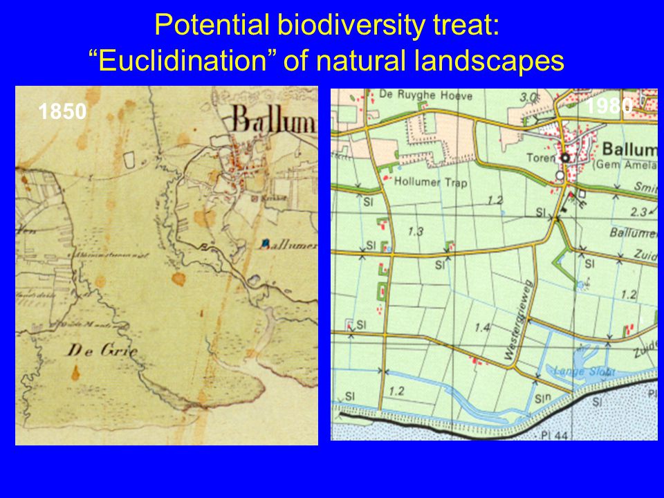
42 Potential biodiversity treat: “Euclidination” of natural landscapes
1980 1850

43 Increasing habitat loss
Separation of effects of habitat loss and habitat fragmentation: Dutch heathland landscapes (9x9 km) 34H - Groote Peel 13H - Elspeet/Gortel h=0.16, D=1.94 h=0.17, D=1.83 10H - Engbertsdijksvenen 06H - Uffelterveen 33H - Groote Heide Increasing habitat loss h=0.10, D=1.92 h=0.10, D=1.82 h=0.09, D=1.72 12H - Notterveen 29H - de Hamert 28H - De Bult 3H - Drouwenerveld h=0.06, D=1.89 h=0.05, D=1.80 h=0.04, D=1.74 h=0.05, D=1.61 Increasing fragmentation

44 The effect is species dependant Diversity of butterflies
2.00 8 8 9 6 12 1.90 12 6 7 7 8 8 9 12 6 10 8 1.80 8 7 8 8 10 7 9 Habitat fractal dimension (D) 4 7 1.70 11 7 7 9 1.60 9 5 4 1.50 5 8 5 5 1.40 1 10 100 Total habitat surface (km2) (after Olff et al)

45 Fragmentation has effect Diversity of breeding birds
2.00 11 12 11 10 12 1.90 11 13 12 10 12 12 12 13 10 12 11 11 1.80 10 11 9 11 12 12 12 Habitat fractal dimension (D) 10 1.70 9 10 11 1.60 11 12 10 10 1.50 8 9 8 7 1.40 1 10 100 Total habitat surface habitat (km2) (after Olff et al.)

46 Species richness vs habitat area and isolation
phytophages parasitoids Tscharntke et al 2000

47 Dispersal assembly theory karakteristieken:
Neutrale theorie Stochastisch, gericht op alle soorten Regionaal en patroongevoelig dispersie paradox

48 The Oak, to gain its present most northerly position in North Britain after being driven out by the cold, probably had to travel fully six hundred miles, and this without external aid would take something like a million years (Reid, 1899)

49 Niche assembly theory karakteristieken:
Uitsluitings beginsel Deterministische competitieve hiërarchie, gericht op dominantie Fitness concept; Beijerinck principe Lokaal Hutchingson’s paradox

50 concurrentie en chaos 1 voedingstof, 2 soorten: 1 winnaar
3 voedingstoffen, 3 soorten: kringetje

51 concurrentie en chaos 3 voedingstoffen, 5 soorten: chaos

52 The null model problem How much of species composition and changes therein can we understand from underlying habitat characteristics (niche assembly) and how much is the mere result of differences in species attributes such as dispersal capacity and longevity (dispersal assembly)

53 Habitat restoratie en Biodiversiteitsherstel

54 Habitat restoratie en Biodiversiteitsherstel

55 Er is nog een derde verklaringsmodel voor hoge biodiversiteit:
Competitie en chaos Kolonisatie en extinctie Hierarchie en schaal

56 Han Olff: schalingsmodel

57 Exclusive spatial niches of species with different body size
Habitat Food Resources Small Species Large Species Exclusive niches

58 Caput biodiversiteit colleges 7+8 De bedreigingen van biodiversiteit

59 Is er sprake van een mondiale biodiversiteitscrisis ?
5-50 millioen species 5-20% bedreigd of extinct laatste paar eeuwen This talk will be structured as follows: first outline the motivation and background problem Then propose a possible solution for the problem Outline the central theory to be developed Introduce the study system and field sites Finally discuss the specific questions that will be adressed Biodiversity gone extinct due to various human activities, where habitat loss is one of the main factors When we want to prevent further species loss, we need to be able to predict where and how we should conserve biodiversity Major problem in predicting biodiversity: Within communities: numerous species interact, nonlinearly, on different spatial and temporal scales Respond to environmental change through heritable information Changes are often irreversable, resulting in a legacy of history Results in complex structures and behaviours

60 Homo sapiens fixes more nitrogen than all other N-fixing organisms together global eutrophication

61 Homo sapiens consumes about 40% of the total global primary production and burns fossil fuels at an equivalent of 10% of the present day biomass global warming

62 Homo sapiens breaks down dispersal barriers as a result of his unprecedented mobility global species mixing

63 Homo sapiens converts natural habitats into agro-ecosystems at an unprecedented rate global species extinctions

64 Current human population density
Cincotta et al. (1999) Nature 404,

65

66

67 % beschermd gebied 3.9 9.250.252 Koude winter woestijnen 7.5
Toendra 3.1 Gematigd naaldbos 0.8 Gematigd grasland 3.2 Gematigd loofbos 4.1 Warme woestijn 9.3 Subtropisch regenwoud 4.7 Tropisch droog bos 5.5 Savanne 5.1 Tropisch regenwoud % beschermd Opp. (km2) bioom

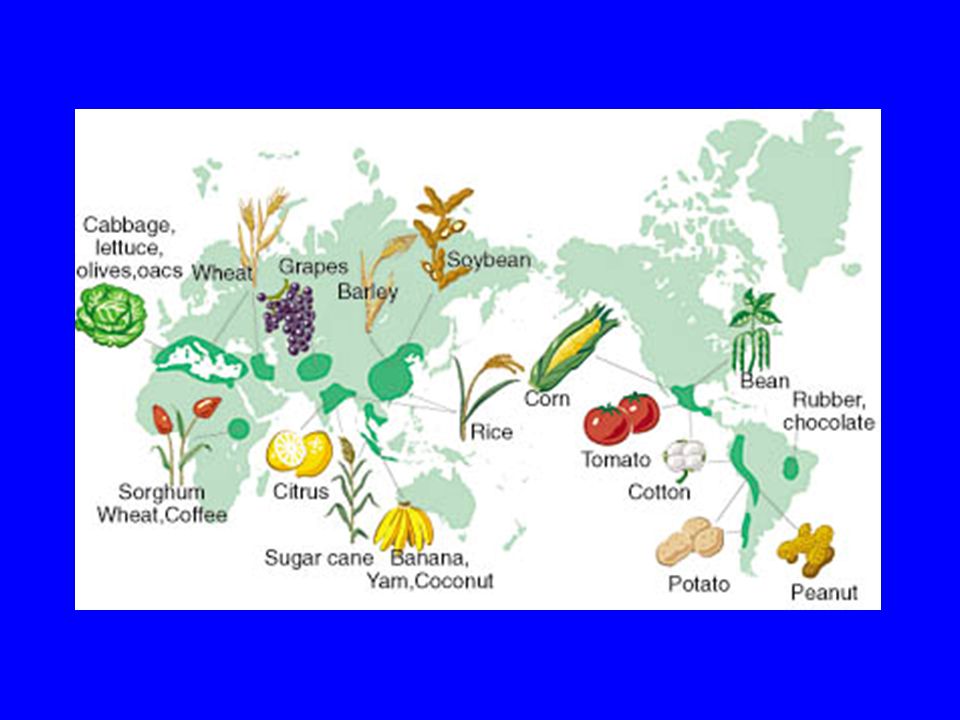
68 25% van alle plantensoorten (80
25% van alle plantensoorten (80.000) worden gekweekt in botanische tuinen. Kew garden alleen heeft al soorten waarvan 10% bedreigde soorten.

69 Meer dan varieteiten van gewassen worden wereldwijd bewaard als zaad in zaadbanken, soms ook als weefsel diepgevroren.

70 3000 diersoorten worden gehouden in zoo’s, 700
3000 diersoorten worden gehouden in zoo’s, individuen in totaal. 900 daarvan kunnen langere tijd worden behouden en daarvan weer slechts een deel in genetisch verantwoorde teeltprogramma’s

71 Ex situ conservering van soorten is minstens 50x zo duur als in situ bescherming van dezelfde soorten binnen hun habitat. Dit bedrag wordt verveelvoudigd als ook aandacht wordt besteed het behoud van voldoende genetische variatie.

72 Voor een duurzame oplossing moeten ecologisch gezonde keuzes worden gemaakt, gebaseerd op begrijpen van de processen die biodiversiteit bepalen

73 Maar er zijn majeure problemen bij het voorspellen van biodiversiteit
Maar er zijn majeure problemen bij het voorspellen van biodiversiteit! Expertise meestal over lokale processen maar de problemen zijn regionaal tot mondiaal.

74 Diversiteit vs habitat
35 total 30 endemic 25 20 number of phyla 15 10 5 freshwater terrestrial marine habitat

75 Holdridge levenszones
evoporatie precipitatie Latitude regio’s Altitude regio’s humidity

76 diversiteit vs verdamping

77 Verdeling soorten potential dominants subordinates
highly adapted to disturbed conditions

78 soorten- vs nutriëntenrijkdom

79 Grime’s model

80 diversiteit vs verstoring

81 diversiteit vs verstoring
species ranking hurricane simulation non-hurricane simulation actual forest data 1 6 12 18 24 30 36 2 5 10 20 50 100 200 500 number of stems/ species / hectare

82

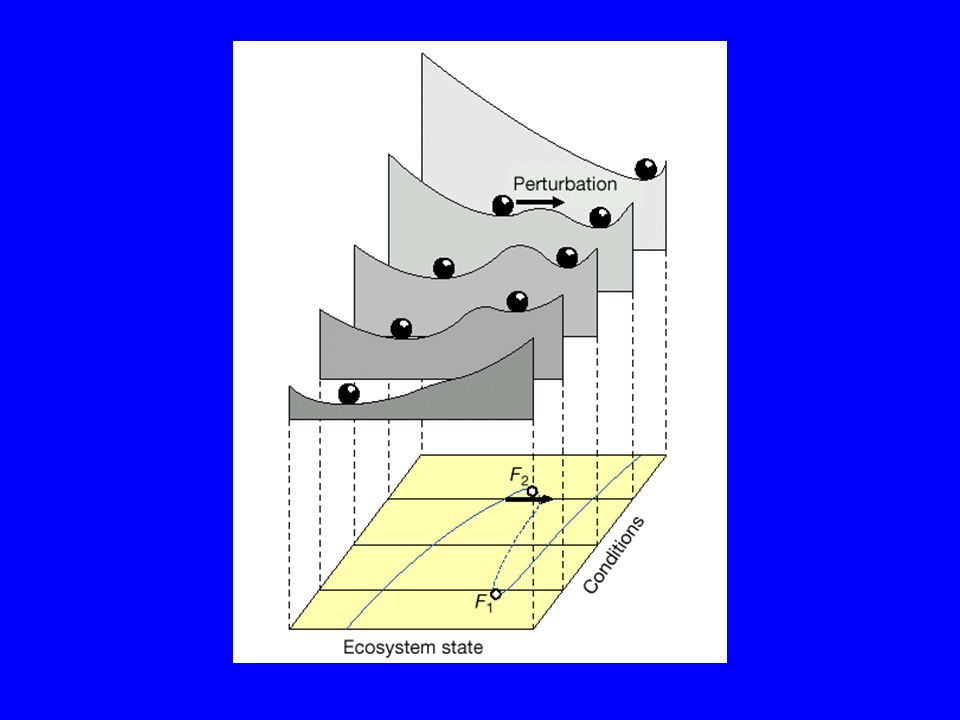
83 Eutrophication of Lake Veluwe
Scheffer et al Nature 2001

84 Scheffer et al Nature 2001